Calibration and validation

This vignette shows how to calibrate and validate a hydrological model

Preparations

Do vignette("run_model_minimalistic") for data loading.

We now need additionally the hydroGOF package.

Note: the warning of deprecated packages can be ignored, openQUARREL is using only non-affected parts of hydroGOF.

library(hydroGOF)
#> Loading required package: zoo
#> 
#> Attaching package: 'zoo'
#> The following objects are masked from 'package:base':
#> 
#>     as.Date, as.Date.numeric
#> The legacy packages maptools, rgdal, and rgeos, underpinning the sp package,
#> which was just loaded, will retire in October 2023.
#> Please refer to R-spatial evolution reports for details, especially
#> https://r-spatial.org/r/2023/05/15/evolution4.html.
#> It may be desirable to make the sf package available;
#> package maintainers should consider adding sf to Suggests:.
#> The sp package is now running under evolution status 2
#>      (status 2 uses the sf package in place of rgdal)
#> Please note that 'maptools' will be retired during October 2023,
#> plan transition at your earliest convenience (see
#> https://r-spatial.org/r/2023/05/15/evolution4.html and earlier blogs
#> for guidance);some functionality will be moved to 'sp'.
#>  Checking rgeos availability: FALSE

… and observed streamflow (column Qmm) from the example data set.

minimum_input <- input_data %>% 
  filter(HSU_ID == "2303") %>% 
  select(DatesR, Qmm) %>%
  inner_join(minimum_input, join_by(DatesR))

Define periods for warm-up, calibration and validation:

# split data set
split_indices <- split_data_set(
  minimum_input,
  c("1981-01-01", "1982-12-31", # warm up
    "1983-01-01", "2000-12-31", # calibration
    "2001-01-01", "2020-12-31") # validation
)

Calibration

Choose the calibration function, the error criterion and streamflow transformation applied (here KGE and none separated by a __), and whether you want to transform parameters to a hypercube.

cal_fn <- "steepest_descent"
error_crit_transfo <- "KGE__none"
do_transfo_param <- TRUE

Put basin information in a list. (todo: some redundancy with input, needs to be solved in future releases)

hydro_data <- list()
hydro_data$BasinObs <- minimum_input
# basin_data is an example data loaded with openQUARREL
minimum_basin_info <- basin_data[["2303"]]
# delete HypsoData not needed here
minimum_basin_info$HypsoData <- NULL
hydro_data$BasinInfo <- minimum_basin_info

Calibrate the model.

# calibrate the model
calibration_results <- calibrate_model(
  hydro_data, split_indices, model, input,
  cal_fn = cal_fn, do_transfo_param = do_transfo_param
) %>% suppressWarnings() %>% suppressMessages()
#> Random sampling with method steepest_descent finished in 1.436 secs with best value 0.77...

Show calibration results:

Calibration finished in 12.564 sec with best criterion 0.8190858 with the model parameters:

# get the parameter names and print
names(calibration_results$model_param) <- names(default_cal_par[[model]]$lower)
print(calibration_results$model_param)
#>        SCF        DDF         Tr         Ts         Tm      LPrat         FC 
#>  1.5000000  0.9071887  1.3200000 -3.0000000 -0.4811310  0.5685123 42.1052038 
#>       BETA         k0         k1         k2       lsuz      cperc       bmax 
#>  2.0492992  1.7360588  7.8950194 30.0000000 11.2260081  0.2955976 30.0000000 
#>     croute 
#> 27.0000000

There is more information after calibration, calibration_results is a list of storing also the used calibration settings cal_par and with more_info the output of the chosen calibration function.

str(calibration_results)
#> List of 12
#>  $ model                 : chr "TUW"
#>  $ snow_module           : NULL
#>  $ model_param           : Named num [1:15] 1.5 0.907 1.32 -3 -0.481 ...
#>   ..- attr(*, "names")= chr [1:15] "SCF" "DDF" "Tr" "Ts" ...
#>  $ preset_snow_parameters: logi FALSE
#>  $ cal_fn                : chr "steepest_descent"
#>  $ error_crit_transfo    : chr "KGE__none"
#>  $ error_crit_val        : num 0.819
#>  $ cal_maximize          : logi TRUE
#>  $ do_transfo_param      : logi TRUE
#>  $ duration              : 'difftime' num 12.564
#>   ..- attr(*, "units")= chr "secs"
#>  $ cal_par               :List of 7
#>   ..$ lower          : Named num [1:15] 0.9 0 1 -3 -2 0 0 0 0 2 ...
#>   .. ..- attr(*, "names")= chr [1:15] "SCF" "DDF" "Tr" "Ts" ...
#>   ..$ upper          : Named num [1:15] 1.5 5 3 1 2 1 600 20 2 30 ...
#>   .. ..- attr(*, "names")= chr [1:15] "SCF" "DDF" "Tr" "Ts" ...
#>   ..$ nof_param      : int 15
#>   ..$ has_snow_module: logi TRUE
#>   ..$ DEoptim        :List of 2
#>   .. ..$ NP     : num 300
#>   .. ..$ itermax: num 200
#>   ..$ malschains     :List of 1
#>   .. ..$ maxEvals: num 2000
#>   ..$ hydroPSO       :List of 1
#>   .. ..$ control:List of 5
#>   .. .. ..$ write2disk: logi FALSE
#>   .. .. ..$ verbose   : logi FALSE
#>   .. .. ..$ npart     : num 80
#>   .. .. ..$ maxit     : num 50
#>   .. .. ..$ reltol    : num 1e-10
#>  $ more_info             :List of 8
#>   ..$ ParamFinalR  : num [1:15] 1 0.181 0.16 0 0.38 ...
#>   ..$ CritFinal    : num -0.819
#>   ..$ NIter        : num 48
#>   ..$ NRuns        : num 1187
#>   ..$ HistParamR   : num [1:48, 1:15] 0.701 0.701 0.701 1 1 ...
#>   .. ..- attr(*, "dimnames")=List of 2
#>   .. .. ..$ : NULL
#>   .. .. ..$ : chr [1:15] "Param1" "Param2" "Param3" "Param4" ...
#>   ..$ HistCrit     : num [1:48, 1] -0.766 -0.789 -0.792 -0.795 -0.797 ...
#>   ..$ CritName     : chr "KGE_none"
#>   ..$ CritBestValue: NULL

Simulate model, similar to vignette("include_snow_module"), but now applying the calibrated parameters.

# simulate snow, if an external snow module is needed (not here, but when you change it)
# todo: this update process can be put in one function
if (exists("snow_module")) {
  if (!is.null(snow_module)) {
    
    # create input
    snow_input <- create_input(snow_module, minimum_input, list()) %>% 
      suppressWarnings() %>% suppressMessages()
    
    # simulate snow
    snow_module_results <- simulate_snow(snow_module, snow_param, snow_input) %>% 
      suppressWarnings() %>% suppressMessages()
    
    # update precip
    input$P <- snow_module_results$surface_water_runoff
    
  }
}

# run model
# Note: we put Qobs as input to have it available for airGR plots
sim <- simulate_model(model, calibration_results$model_param, input, Qobs = hydro_data$BasinObs$Qmm)

# merge snow module results with hydro model results
if (exists("snow_module_results")) {
  sim <- merge_snow_runoff_sim(sim, snow_module_results) 
}

Validation

Plots

For validation there are two plots available which can be right now only only saved to disc as pdf (which will be changed in a future release).

The first is a simple plot showing simulated and observed streamflow with some indicators for both the calibration and validation period, simulated streamflow is red.

# define and create a output folder
output_folder <- "output"
dir.create(output_folder)

save_cal_val_plot(file.path(output_folder, "cal_val_plot.pdf"), hydro_data$BasinObs, sim$Qsim, split_indices)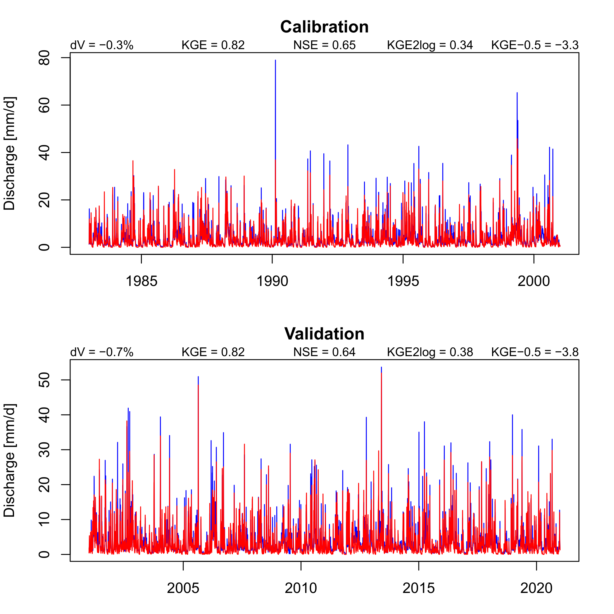

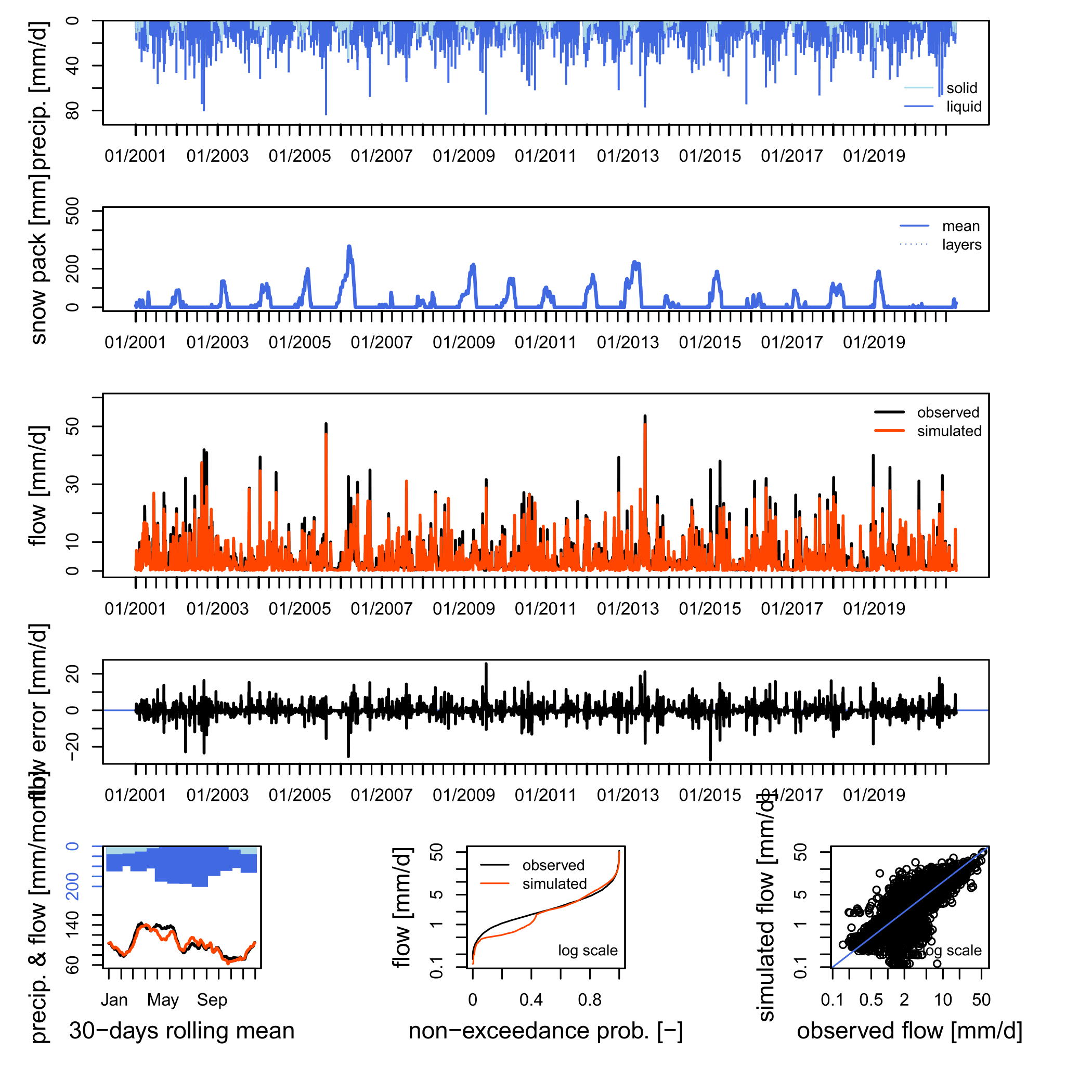
The second plot is the great airGR::plot adapted to models from other packages. We plot it for the calibration and validation period separately.

# airGR plots for validation and calibration time period

# calibration period
save_airGR_plot(file.path(output_folder, "airGR_cal.pdf"), model, sim, split_indices$ind_cal, hydro_data) %>% 
  suppressWarnings() %>% suppressMessages()
# validation period
save_airGR_plot(file.path(output_folder, "airGR_val.pdf"), model, sim, split_indices$ind_val, hydro_data) %>% 
  suppressWarnings() %>% suppressMessages()

Here is the validation plot shown:

It seems that this model has difficulties in spring with snow melt, quite probably because of a missing snow covered fraction parameterisation. Try this with the model CemaNeigeGR4J as this snow module has such a parameterisation implemented.

Calculation of (sub)seasonal performance metrics

Define metrics with streamflow transformations, separated by __. For example mae__power__-0.5 is the mean absolute error calculated with hydroGOF::mae, and using a power transformation with exponent -0.5.

Note: All these (and other) string combinations can also be used for calibration with applying it to error_crit_transfo.

# validation settings
val_crit_transfo <- c("KGE__none", "NSE__none", "VE__none", "pbias__none", "mae__none", "mse__none",
                      "KGE__power__0.2",  "NSE__power__0.2", "mae__power__0.2", "mse__power__0.2",
                      "KGE__boxcoxsantos", "NSE__boxcoxsantos", "mae__boxcoxsantos", "mse__boxcoxsantos",
                      "KGEtang__log", "NSE__log", "mae__log", "mse__log",
                      "KGE__power__-0.5", "NSE__power__-0.5", "mae__power__-0.5", "mse__power__-0.5")

Define the subseasons for which the above defined metrics are calculated for:

# a list with names and arrays of two digits describing months used to calculate
# subseasonal validation metrics
val_subseason <- list(spring = c("02", "03", "04", "05"), 
                      summer = c("06", "07", "08", "09"))

Calculate (sub)seasonal metrics. It will automatically calculate performance metrics for the whole year (all).

# calculate performance metrics for calibration period
perf_cal <- calc_subseasonal_validation_results(val_subseason, hydro_data$BasinObs$DatesR,
                                                split_indices$ind_cal, "calibration",
                                                col_name = "period",
                                                sim$Qsim, hydro_data$BasinObs$Qmm, val_crit_transfo
)

# calculate performance metrics for calibration period
perf_val <- calc_subseasonal_validation_results(val_subseason, hydro_data$BasinObs$DatesR,
                                                split_indices$ind_val, "validation",
                                                col_name = "period",
                                                sim$Qsim, hydro_data$BasinObs$Qmm, val_crit_transfo
)

# combine periods in one data frame
perf_df <- dplyr::bind_rows(perf_cal, perf_val)

Show the results which is a tibble. Lambda is the exponent if a power transformation is used …

knitr::kable(head(perf_df))

crit	transfo	lambda	value	season	period
KGE	none	NA	0.7944523	spring	calibration
NSE	none	NA	0.6088709	spring	calibration
VE	none	NA	0.5687535	spring	calibration
pbias	none	NA	4.2000000	spring	calibration
mae	none	NA	1.9489648	spring	calibration
mse	none	NA	9.9249006	spring	calibration

This result can be stored as ascii file:

# write ascii results overview
write_ascii(
  file.path(output_folder, "perf_ascii.txt"),
  # to include also the parameters
  calibration_results, 
  perf_df
)

All results can be stored as a binary

# for this split sim in calibration and validation periods
sim_list <- list()
sim_list$cal <- subset_simulations(split_indices$ind_cal, sim)
sim_list$val <- subset_simulations(split_indices$ind_val, sim)

saveRDS(
  list(
    calibration = calibration_results,
    simulation_val = sim_list$val,
    simulation_cal = sim_list$cal,
    sim_more_info = sim_list$more_info,
    validation = perf_df
  ),
  file.path(output_folder, "results_binary.rds")
)

Next steps

Choose a different model, or a snow module/hydrological model combination, or a different calibration function (see vignette("calibration_methods_overview") for a complete list), or a different streamflow transformation for calibration (e.g. error_crit_transfo <- "NSE__power__0.2") or do it in a different subbasin with filtering the example data to a different HSU_ID.

Michael Schirmer

2025-08-25